


« Prev Next »
Once you have performed an experiment, how can you tell if your results are significant? For example, say that you are performing a genetic cross in which you know the genotypes of the parents. In this situation, you might hypothesize that the cross will result in a certain ratio of phenotypes in the offspring. But what if your observed results do not exactly match your expectations? How can you tell whether this deviation was due to chance? The key to answering these questions is the use of statistics, which allows you to determine whether your data are consistent with your hypothesis.
Forming and Testing a Hypothesis
The first thing any scientist does before performing an experiment is to form a hypothesis about the experiment's outcome. This often takes the form of a null hypothesis, which is a statistical hypothesis that states there will be no difference between observed and expected data. The null hypothesis is proposed by a scientist before completing an experiment, and it can be either supported by data or disproved in favor of an alternate hypothesis.
Let's consider some examples of the use of the null hypothesis in a genetics experiment. Remember that Mendelian inheritance deals with traits that show discontinuous variation, which means that the phenotypes fall into distinct categories. As a consequence, in a Mendelian genetic cross, the null hypothesis is usually an extrinsic hypothesis; in other words, the expected proportions can be predicted and calculated before the experiment starts. Then an experiment can be designed to determine whether the data confirm or reject the hypothesis. On the other hand, in another experiment, you might hypothesize that two genes are linked. This is called an intrinsic hypothesis, which is a hypothesis in which the expected proportions are calculated after the experiment is done using some information from the experimental data (McDonald, 2008).
How Math Merged with Biology
But how did mathematics and genetics come to be linked through the use of hypotheses and statistical analysis? The key figure in this process was Karl Pearson, a turn-of-the-century mathematician who was fascinated with biology. When asked what his first memory was, Pearson responded by saying, "Well, I do not know how old I was, but I was sitting in a high chair and I was sucking my thumb. Someone told me to stop sucking it and said that if I did so, the thumb would wither away. I put my two thumbs together and looked at them a long time. ‘They look alike to me,' I said to myself, ‘I can't see that the thumb I suck is any smaller than the other. I wonder if she could be lying to me'" (Walker, 1958). As this anecdote illustrates, Pearson was perhaps born to be a scientist. He was a sharp observer and intent on interpreting his own data. During his career, Pearson developed statistical theories and applied them to the exploration of biological data. His innovations were not well received, however, and he faced an arduous struggle in convincing other scientists to accept the idea that mathematics should be applied to biology. For instance, during Pearson's time, the Royal Society, which is the United Kingdom's academy of science, would accept papers that concerned either mathematics or biology, but it refused to accept papers than concerned both subjects (Walker, 1958). In response, Pearson, along with Francis Galton and W. F. R. Weldon, founded a new journal called Biometrika in 1901 to promote the statistical analysis of data on heredity. Pearson's persistence paid off. Today, statistical tests are essential for examining biological data.
Pearson's Chi-Square Test for Goodness-of-Fit
One of Pearson's most significant achievements occurred in 1900, when he developed a statistical test called Pearson's chi-square (Χ2) test, also known as the chi-square test for goodness-of-fit (Pearson, 1900). Pearson's chi-square test is used to examine the role of chance in producing deviations between observed and expected values. The test depends on an extrinsic hypothesis, because it requires theoretical expected values to be calculated. The test indicates the probability that chance alone produced the deviation between the expected and the observed values (Pierce, 2005). When the probability calculated from Pearson's chi-square test is high, it is assumed that chance alone produced the difference. Conversely, when the probability is low, it is assumed that a significant factor other than chance produced the deviation.
In 1912, J. Arthur Harris applied Pearson's chi-square test to examine Mendelian ratios (Harris, 1912). It is important to note that when Gregor Mendel studied inheritance, he did not use statistics, and neither did Bateson, Saunders, Punnett, and Morgan during their experiments that discovered genetic linkage. Thus, until Pearson's statistical tests were applied to biological data, scientists judged the goodness of fit between theoretical and observed experimental results simply by inspecting the data and drawing conclusions (Harris, 1912). Although this method can work perfectly if one's data exactly matches one's predictions, scientific experiments often have variability associated with them, and this makes statistical tests very useful.
The chi-square value is calculated using the following formula:
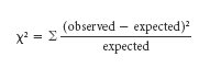
Using this formula, the difference between the observed and expected frequencies is calculated for each experimental outcome category. The difference is then squared and divided by the expected frequency. Finally, the chi-square values for each outcome are summed together, as represented by the summation sign (Σ).
Pearson's chi-square test works well with genetic data as long as there are enough expected values in each group. In the case of small samples (less than 10 in any category) that have 1 degree of freedom, the test is not reliable. (Degrees of freedom, or df, will be explained in full later in this article.) However, in such cases, the test can be corrected by using the Yates correction for continuity, which reduces the absolute value of each difference between observed and expected frequencies by 0.5 before squaring. Additionally, it is important to remember that the chi-square test can only be applied to numbers of progeny, not to proportions or percentages.
Now that you know the rules for using the test, it's time to consider an example of how to calculate Pearson's chi-square. Recall that when Mendel crossed his pea plants, he learned that tall (T) was dominant to short (t). You want to confirm that this is correct, so you start by formulating the following null hypothesis: In a cross between two heterozygote (Tt) plants, the offspring should occur in a 3:1 ratio of tall plants to short plants. Next, you cross the plants, and after the cross, you measure the characteristics of 400 offspring. You note that there are 305 tall pea plants and 95 short pea plants; these are your observed values. Meanwhile, you expect that there will be 300 tall plants and 100 short plants from the Mendelian ratio.
You are now ready to perform statistical analysis of your results, but first, you have to choose a critical value at which to reject your null hypothesis. You opt for a critical value probability of 0.01 (1%) that the deviation between the observed and expected values is due to chance. This means that if the probability is less than 0.01, then the deviation is significant and not due to chance, and you will reject your null hypothesis. However, if the deviation is greater than 0.01, then the deviation is not significant and you will not reject the null hypothesis.
So, should you reject your null hypothesis or not? Here's a summary of your observed and expected data:
| Tall | Short | |
| Expected | 300 | 100 |
| Observed | 305 | 95 |
Now, let's calculate Pearson's chi-square:
- For tall plants: Χ2 = (305 - 300)2 / 300 = 0.08
- For short plants: Χ2 = (95 - 100)2 / 100 = 0.25
- The sum of the two categories is 0.08 + 0.25 = 0.33
- Therefore, the overall Pearson's chi-square for the experiment is Χ2 = 0.33
Next, you determine the probability that is associated with your calculated chi-square value. To do this, you compare your calculated chi-square value with theoretical values in a chi-square table that has the same number of degrees of freedom. Degrees of freedom represent the number of ways in which the observed outcome categories are free to vary. For Pearson's chi-square test, the degrees of freedom are equal to n - 1, where n represents the number of different expected phenotypes (Pierce, 2005). In your experiment, there are two expected outcome phenotypes (tall and short), so n = 2 categories, and the degrees of freedom equal 2 - 1 = 1. Thus, with your calculated chi-square value (0.33) and the associated degrees of freedom (1), you can determine the probability by using a chi-square table (Table 1).
Table 1: Chi-Square Table
|
Degrees of Freedom (df) |
Probability (P) | |||||||||
| 0.995 | 0.99 | 0.975 | 0.95 | 0.90 | 0.10 | 0.05 | 0.025 | 0.01 | 0.005 | |
| 1 | --- | --- | 0.001 | 0.004 | 0.016 | 2.706 | 3.841 | 5.024 | 6.635 | 7.879 |
| 2 | 0.010 | 0.020 | 0.051 | 0.103 | 0.211 | 4.605 | 5.991 | 7.378 | 9.210 | 10.597 |
| 3 | 0.072 | 0.115 | 0.216 | 0.352 | 0.584 | 6.251 | 7.815 | 9.348 | 11.345 | 12.838 |
| 4 | 0.207 | 0.297 | 0.484 | 0.711 | 1.064 | 7.779 | 9.488 | 11.143 | 13.277 | 14.860 |
| 5 | 0.412 | 0.554 | 0.831 | 1.145 | 1.610 | 9.236 | 11.070 | 12.833 | 15.086 | 16.750 |
| 6 | 0.676 | 0.872 | 1.237 | 1.635 | 2.204 | 10.645 | 12.592 | 14.449 | 16.812 | 18.548 |
| 7 | 0.989 | 1.239 | 1.690 | 2.167 | 2.833 | 12.017 | 14.067 | 16.013 | 18.475 | 20.278 |
| 8 | 1.344 | 1.646 | 2.180 | 2.733 | 3.490 | 13.362 | 15.507 | 17.535 | 20.090 | 21.955 |
| 9 | 1.735 | 2.088 | 2.700 | 3.325 | 4.168 | 14.684 | 16.919 | 19.023 | 21.666 | 23.589 |
| 10 | 2.156 | 2.558 | 3.247 | 3.940 | 4.865 | 15.987 | 18.307 | 20.483 | 23.209 | 25.188 |
| 11 | 2.603 | 3.053 | 3.816 | 4.575 | 5.578 | 17.275 | 19.675 | 21.920 | 24.725 | 26.757 |
| 12 | 3.074 | 3.571 | 4.404 | 5.226 | 6.304 | 18.549 | 21.026 | 23.337 | 26.217 | 28.300 |
| 13 | 3.565 | 4.107 | 5.009 | 5.892 | 7.042 | 19.812 | 22.362 | 24.736 | 27.688 | 29.819 |
| 14 | 4.075 | 4.660 | 5.629 | 6.571 | 7.790 | 21.064 | 23.685 | 26.119 | 29.141 | 31.319 |
| 15 | 4.601 | 5.229 | 6.262 | 7.261 | 8.547 | 22.307 | 24.996 | 27.488 | 30.578 | 32.801 |
| 16 | 5.142 | 5.812 | 6.908 | 7.962 | 9.312 | 23.542 | 26.296 | 28.845 | 32.000 | 34.267 |
| 17 | 5.697 | 6.408 | 7.564 | 8.672 | 10.085 | 24.769 | 27.587 | 30.191 | 33.409 | 35.718 |
| 18 | 6.265 | 7.015 | 8.231 | 9.390 | 10.865 | 25.989 | 28.869 | 31.526 | 34.805 | 37.156 |
| 19 | 6.844 | 7.633 | 8.907 | 10.117 | 11.651 | 27.204 | 30.144 | 32.852 | 36.191 | 38.582 |
| 20 | 7.434 | 8.260 | 9.591 | 10.851 | 12.443 | 28.412 | 31.410 | 34.170 | 37.566 | 39.997 |
| 21 | 8.034 | 8.897 | 10.283 | 11.591 | 13.240 | 29.615 | 32.671 | 35.479 | 38.932 | 41.401 |
| 22 | 8.643 | 9.542 | 10.982 | 12.338 | 14.041 | 30.813 | 33.924 | 36.781 | 40.289 | 42.796 |
| 23 | 9.260 | 10.196 | 11.689 | 13.091 | 14.848 | 32.007 | 35.172 | 38.076 | 41.638 | 44.181 |
| 24 | 9.886 | 10.856 | 12.401 | 13.848 | 15.659 | 33.196 | 36.415 | 39.364 | 42.980 | 45.559 |
| 25 | 10.520 | 11.524 | 13.120 | 14.611 | 16.473 | 34.382 | 37.652 | 40.646 | 44.314 | 46.928 |
| 26 | 11.160 | 12.198 | 13.844 | 15.379 | 17.292 | 35.563 | 38.885 | 41.923 | 45.642 | 48.290 |
| 27 | 11.808 | 12.879 | 14.573 | 16.151 | 18.114 | 36.741 | 40.113 | 43.195 | 46.963 | 49.645 |
| 28 | 12.461 | 13.565 | 15.308 | 16.928 | 18.939 | 37.916 | 41.337 | 44.461 | 48.278 | 50.993 |
| 29 | 13.121 | 14.256 | 16.047 | 17.708 | 19.768 | 39.087 | 42.557 | 45.722 | 49.588 | 52.336 |
| 30 | 13.787 | 14.953 | 16.791 | 18.493 | 20.599 | 40.256 | 43.773 | 46.979 | 50.892 | 53.672 |
| 40 | 20.707 | 22.164 | 24.433 | 26.509 | 29.051 | 51.805 | 55.758 | 59.342 | 63.691 | 66.766 |
| 50 | 27.991 | 29.707 | 32.357 | 34.764 | 37.689 | 63.167 | 67.505 | 71.420 | 76.154 | 79.490 |
| 60 | 35.534 | 37.485 | 40.482 | 43.188 | 46.459 | 74.397 | 79.082 | 83.298 | 88.379 | 91.952 |
| 70 | 43.275 | 45.442 | 48.758 | 51.739 | 55.329 | 85.527 | 90.531 | 95.023 | 100.425 | 104.215 |
| 80 | 51.172 | 53.540 | 57.153 | 60.391 | 64.278 | 96.578 | 101.879 | 106.629 | 112.329 | 116.321 |
| 90 | 59.196 | 61.754 | 65.647 | 69.126 | 73.291 | 107.565 | 113.145 | 118.136 | 124.116 | 128.299 |
| 100 | 67.328 | 70.065 | 74.222 | 77.929 | 82.358 | 118.498 | 124.342 | 129.561 | 135.807 | 140.169 |
|
Not Significant & Do Not Reject Hypothesis
|
Significant & Reject Hypothesis | |||||||||
(Table adapted from Jones, 2008)
Note that the chi-square table is organized with degrees of freedom (df) in the left column and probabilities (P) at the top. The chi-square values associated with the probabilities are in the center of the table. To determine the probability, first locate the row for the degrees of freedom for your experiment, then determine where the calculated chi-square value would be placed among the theoretical values in the corresponding row.
At the beginning of your experiment, you decided that if the probability was less than 0.01, you would reject your null hypothesis because the deviation would be significant and not due to chance. Now, looking at the row that corresponds to 1 degree of freedom, you see that your calculated chi-square value of 0.33 falls between 0.016, which is associated with a probability of 0.9, and 2.706, which is associated with a probability of 0.10. Therefore, there is between a 10% and 90% probability that the deviation you observed between your expected and the observed numbers of tall and short plants is due to chance. In other words, the probability associated with your chi-square value is much greater than the critical value of 0.01. This means that we will not reject our null hypothesis, and the deviation between the observed and expected results is not significant.
Level of Significance
Determining whether to accept or reject a hypothesis is decided by the experimenter, who is the person who chooses the "level of significance" or confidence. Scientists commonly use the 0.05, 0.01, or 0.001 probability levels as cut-off values. For instance, in the example experiment, you used the 0.01 probability. Thus, P ≥ 0.01 can be interpreted to mean that chance likely caused the deviation between the observed and the expected values (i.e. there is a greater than 1% probability that chance explains the data). If instead we had observed that P ≤ 0.01, this would mean that there is less than a 1% probability that our data can be explained by chance. There is a significant difference between our expected and observed results, so the deviation must be caused by something other than chance.
References and Recommended Reading
Harris, J. A. A simple test of the goodness of fit of Mendelian ratios. American Naturalist 46, 741–745 (1912)
Jones, J. "Table: Chi-Square Probabilities." http://people.richland.edu/james/lecture/m170/tbl-chi.html (2008) (accessed July 7, 2008)
McDonald, J. H. Chi-square test for goodness-of-fit. From The Handbook of Biological Statistics. http://udel.edu/~mcdonald/statchigof.html (2008) (accessed June 9, 2008)
Pearson, K. On the criterion that a given system of deviations from the probable in the case of correlated system of variables is such that it can be reasonably supposed to have arisen from random sampling. Philosophical Magazine 50, 157–175 (1900)
Pierce, B. Genetics: A Conceptual Approach (New York, Freeman, 2005)
Walker, H. M. The contributions of Karl Pearson. Journal of the American Statistical Association 53, 11–22 (1958)